null
子地块
当我们想在同一个图形中显示两个或多个绘图时,需要使用子绘图。我们可以使用两种稍有不同的方法以两种方式进行。 方法1
python
# importing required modules import matplotlib.pyplot as plt import numpy as np # function to generate coordinates def create_plot(ptype): # setting the x-axis values x = np.arange( - 10 , 10 , 0.01 ) # setting the y-axis values if ptype = = 'linear' : y = x elif ptype = = 'quadratic' : y = x * * 2 elif ptype = = 'cubic' : y = x * * 3 elif ptype = = 'quartic' : y = x * * 4 return (x, y) # setting a style to use plt.style.use( 'fivethirtyeight' ) # create a figure fig = plt.figure() # define subplots and their positions in figure plt1 = fig.add_subplot( 221 ) plt2 = fig.add_subplot( 222 ) plt3 = fig.add_subplot( 223 ) plt4 = fig.add_subplot( 224 ) # plotting points on each subplot x, y = create_plot( 'linear' ) plt1.plot(x, y, color = 'r' ) plt1.set_title( '$y_1 = x$' ) x, y = create_plot( 'quadratic' ) plt2.plot(x, y, color = 'b' ) plt2.set_title( '$y_2 = x^2$' ) x, y = create_plot( 'cubic' ) plt3.plot(x, y, color = 'g' ) plt3.set_title( '$y_3 = x^3$' ) x, y = create_plot( 'quartic' ) plt4.plot(x, y, color = 'k' ) plt4.set_title( '$y_4 = x^4$' ) # adjusting space between subplots fig.subplots_adjust(hspace = . 5 ,wspace = 0.5 ) # function to show the plot plt.show() |
输出:
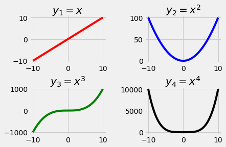
让我们一步一步地完成这个计划:
plt.style.use('fivethirtyeight')
- 可以通过设置不同的可用样式或设置自己的样式来配置打印样式。您可以了解有关此功能的更多信息 在这里
fig = plt.figure()
- Figure充当所有绘图元素的顶级容器。所以,我们把一个数字定义为 无花果 它将包含我们所有的子地块。
plt1 = fig.add_subplot(221)plt2 = fig.add_subplot(222)plt3 = fig.add_subplot(223)plt4 = fig.add_subplot(224)
- 这里我们使用fig.add_子图方法来定义子图及其位置。功能原型如下所示:
add_subplot(nrows, ncols, plot_number)
- 如果一个子图应用于一个图形,则该图形在概念上将被拆分为“nrows”*“ncols”子轴。参数“plot_number”标识函数调用必须创建的子图“绘图编号”的范围从1到最大值为“nrows”*“ncols”。 如果三个参数的值小于10,则可以使用一个int参数调用函数子图,其中数百个表示“nrows”,十个表示“ncols”,单位表示“plot_number”。这意味着:而不是 子地块(2,3,4) 我们可以写作 子地块(234) . 该图将明确说明如何指定位置:
![图片[2]-用Python |集2绘制图形-yiteyi-C++库](https://media.geeksforgeeks.org/wp-content/cdn-uploads/20210722193312/sub11.png)
x, y = create_plot('linear')plt1.plot(x, y, color ='r')plt1.set_title('$y_1 = x$')
- 接下来,我们在每个子地块上绘制点。首先,我们使用 创建_图 通过指定我们想要的曲线类型来实现。 然后,我们使用 情节 方法子地块的标题通过使用 设置标题 方法使用 $ 在标题的开头和结尾,文本将确保“u”(下划线)作为下标,而“^”作为上标。
fig.subplots_adjust(hspace=.5,wspace=0.5)
- 这是另一种在子地块之间创建空间的实用方法。
plt.show()
- 最后,我们称之为plt。show()方法,该方法将显示当前图形。
方法2
python
# importing required modules import matplotlib.pyplot as plt import numpy as np # function to generate coordinates def create_plot(ptype): # setting the x-axis values x = np.arange( 0 , 5 , 0.01 ) # setting y-axis values if ptype = = 'sin' : # a sine wave y = np.sin( 2 * np.pi * x) elif ptype = = 'exp' : # negative exponential function y = np.exp( - x) elif ptype = = 'hybrid' : # a damped sine wave y = (np.sin( 2 * np.pi * x)) * (np.exp( - x)) return (x, y) # setting a style to use plt.style.use( 'ggplot' ) # defining subplots and their positions plt1 = plt.subplot2grid(( 11 , 1 ), ( 0 , 0 ), rowspan = 3 , colspan = 1 ) plt2 = plt.subplot2grid(( 11 , 1 ), ( 4 , 0 ), rowspan = 3 , colspan = 1 ) plt3 = plt.subplot2grid(( 11 , 1 ), ( 8 , 0 ), rowspan = 3 , colspan = 1 ) # plotting points on each subplot x, y = create_plot( 'sin' ) plt1.plot(x, y, label = 'sine wave' , color = 'b' ) x, y = create_plot( 'exp' ) plt2.plot(x, y, label = 'negative exponential' , color = 'r' ) x, y = create_plot( 'hybrid' ) plt3.plot(x, y, label = 'damped sine wave' , color = 'g' ) # show legends of each subplot plt1.legend() plt2.legend() plt3.legend() # function to show plot plt.show() |
输出:
![图片[3]-用Python |集2绘制图形-yiteyi-C++库](https://media.geeksforgeeks.org/wp-content/cdn-uploads/20210722193347/sub3.png)
我们也来看看这个项目的重要部分:
plt1 = plt.subplot2grid((11,1), (0,0), rowspan = 3, colspan = 1)plt2 = plt.subplot2grid((11,1), (4,0), rowspan = 3, colspan = 1)plt3 = plt.subplot2grid((11,1), (8,0), rowspan = 3, colspan = 1)
- 子地块2网格 类似于“pyplot.subplot”,但使用基于0的索引,并让子Plot占据多个单元格。 让我们试着理解 子地块2网格 方法: 1.论点1:网格的几何结构 2.论点2:子地块在网格中的位置 3.论点3:(行范围)子地块覆盖的行数。 4.论据4:(colspan)子地块覆盖的柱数。 这个数字将使这个概念更加清晰:
![图片[4]-用Python |集2绘制图形-yiteyi-C++库](https://media.geeksforgeeks.org/wp-content/cdn-uploads/20210722193421/sub4.png)
- 在我们的示例中,每个子地块跨越3行和1列,其中有两个空行(第4、8行)。
x, y = create_plot('sin')plt1.plot(x, y, label = 'sine wave', color ='b')
- 这部分没有什么特别之处,因为在子图上绘制点的语法保持不变。
plt1.legend()
- 这将在图上显示子批次的标签。
plt.show()
- 最后,我们称之为plt。show()函数显示当前绘图。
注: 通过以上两个例子,我们可以推断应该使用 子地块() 方法,当图的大小一致时 subplot2grid() 当我们想要在子地块的位置和大小上有更多的灵活性时,应该首选这种方法。
三维绘图
我们可以很容易地在matplotlib中绘制三维图形。现在,我们讨论一些重要的和常用的三维图。
- 绘图点
python
from mpl_toolkits.mplot3d import axes3d import matplotlib.pyplot as plt from matplotlib import style import numpy as np # setting a custom style to use style.use( 'ggplot' ) # create a new figure for plotting fig = plt.figure() # create a new subplot on our figure # and set projection as 3d ax1 = fig.add_subplot( 111 , projection = '3d' ) # defining x, y, z co-ordinates x = np.random.randint( 0 , 10 , size = 20 ) y = np.random.randint( 0 , 10 , size = 20 ) z = np.random.randint( 0 , 10 , size = 20 ) # plotting the points on subplot # setting labels for the axes ax1.set_xlabel( 'x-axis' ) ax1.set_ylabel( 'y-axis' ) ax1.set_zlabel( 'z-axis' ) # function to show the plot plt.show() |
- 上述程序的输出将为您提供一个可以旋转或放大绘图的窗口。这里是一个屏幕截图:(暗点比亮点更近)
![图片[5]-用Python |集2绘制图形-yiteyi-C++库](https://www.yiteyi.com/wp-content/uploads/geeks/20210722/geeks_figure_1-1.png)
- 现在让我们试着了解一下这段代码的一些重要方面。
from mpl_toolkits.mplot3d import axes3d
- 这是在三维空间上绘图所需的模块。
ax1 = fig.add_subplot(111, projection='3d')
- 在这里,我们在图形上创建一个子图,并将投影参数设置为3d。
ax1.scatter(x, y, z, c = 'm', marker = 'o')
- 现在我们使用 .散布 函数在XYZ平面上绘制点。
- 绘制线
python
# importing required modules from mpl_toolkits.mplot3d import axes3d import matplotlib.pyplot as plt from matplotlib import style import numpy as np # setting a custom style to use style.use( 'ggplot' ) # create a new figure for plotting fig = plt.figure() # create a new subplot on our figure ax1 = fig.add_subplot( 111 , projection = '3d' ) # defining x, y, z co-ordinates x = np.random.randint( 0 , 10 , size = 5 ) y = np.random.randint( 0 , 10 , size = 5 ) z = np.random.randint( 0 , 10 , size = 5 ) # plotting the points on subplot ax1.plot_wireframe(x,y,z) # setting the labels ax1.set_xlabel( 'x-axis' ) ax1.set_ylabel( 'y-axis' ) ax1.set_zlabel( 'z-axis' ) plt.show() |
- 上述程序的三维绘图截图如下所示:
![图片[6]-用Python |集2绘制图形-yiteyi-C++库](https://media.geeksforgeeks.org/wp-content/cdn-uploads/20210722193517/figure_1.png)
- 本课程与前一课程的主要区别在于:
ax1.plot_wireframe(x,y,z)
- 我们曾经 .plot_线框() 方法在给定的一组三维点上绘制线。
- 绘图条
python
# importing required modules from mpl_toolkits.mplot3d import axes3d import matplotlib.pyplot as plt from matplotlib import style import numpy as np # setting a custom style to use style.use( 'ggplot' ) # create a new figure for plotting fig = plt.figure() # create a new subplot on our figure ax1 = fig.add_subplot( 111 , projection = '3d' ) # defining x, y, z co-ordinates for bar position x = [ 1 , 2 , 3 , 4 , 5 , 6 , 7 , 8 , 9 , 10 ] y = [ 4 , 3 , 1 , 6 , 5 , 3 , 7 , 5 , 3 , 7 ] z = np.zeros( 10 ) # size of bars dx = np.ones( 10 ) # length along x-axis dy = np.ones( 10 ) # length along y-axs dz = [ 1 , 3 , 4 , 2 , 6 , 7 , 5 , 5 , 10 , 9 ] # height of bar # setting color scheme color = [] for h in dz: if h > 5 : color.append( 'r' ) else : color.append( 'b' ) # plotting the bars ax1.bar3d(x, y, z, dx, dy, dz, color = color) # setting axes labels ax1.set_xlabel( 'x-axis' ) ax1.set_ylabel( 'y-axis' ) ax1.set_zlabel( 'z-axis' ) plt.show() |
- 创建的三维环境截图如下:
![图片[7]-用Python |集2绘制图形-yiteyi-C++库](https://media.geeksforgeeks.org/wp-content/cdn-uploads/20210722193545/figure_1-2.png)
- 让我们来看看这个项目的重要方面:
x = [1,2,3,4,5,6,7,8,9,10]y = [4,3,1,6,5,3,7,5,3,7]z = np.zeros(10)
- 这里,我们定义了杆的基本位置。设置z=0意味着所有钢筋都从XY平面开始。
dx = np.ones(10) # length along x-axisdy = np.ones(10) # length along y-axsdz = [1,3,4,2,6,7,5,5,10,9] # height of bar
- dx,dy,dz表示棒材的尺寸。将其视为长方体,DX、DY、DZ分别沿X、Y、Z轴展开。
for h in dz: if h > 5: color.append('r') else: color.append('b')
- 在这里,我们将每个条的颜色设置为列表。对于高度大于5的条,颜色方案为红色,否则为蓝色。
ax1.bar3d(x, y, z, dx, dy, dz, color = color)
- 最后,我们使用 .bar3d() 作用
- 绘制曲线
python
# importing required modules from mpl_toolkits.mplot3d import axes3d import matplotlib.pyplot as plt from matplotlib import style import numpy as np # setting a custom style to use style.use( 'ggplot' ) # create a new figure for plotting fig = plt.figure() # create a new subplot on our figure ax1 = fig.add_subplot( 111 , projection = '3d' ) # get points for a mesh grid u, v = np.mgrid[ 0 : 2 * np.pi: 200j , 0 :np.pi: 100j ] # setting x, y, z co-ordinates x = np.cos(u) * np.sin(v) y = np.sin(u) * np.sin(v) z = np.cos(v) # plotting the curve ax1.plot_wireframe(x, y, z, rstride = 5 , cstride = 5 , linewidth = 1 ) plt.show() |
- 该程序的输出如下所示:
![图片[8]-用Python |集2绘制图形-yiteyi-C++库](https://www.yiteyi.com/wp-content/uploads/geeks/20210722/geeks_figure_1-31.png)
- 在这里,我们绘制了一个球体作为网格。 让我们来看一些重要的部分:
u, v = np.mgrid[0:2*np.pi:200j, 0:np.pi:100j]
- 我们使用np。mgrid以获取点,以便我们可以创建网格。 你可以阅读更多关于这方面的内容 在这里 .
x=np.cos(u)*np.sin(v)y=np.sin(u)*np.sin(v)z=np.cos(v)
- 这只是一个球体的参数方程。
ax1.plot_wireframe(x, y, z, rstride = 5, cstride = 5, linewidth = 1)
- 阿甘,我们用 .plot_线框() 方法在这里 斯特里德 和 驾驶 参数可以用来设置网格的密度。
下一篇文章: Python |集3中的图形绘制 本文由 尼希尔·库马尔 .如果你喜欢GeekSforgeks并想贡献自己的力量,你也可以用write写一篇文章。极客。组织或邮寄你的文章进行评论-team@geeksforgeeks.org.看到你的文章出现在Geeksforgeks主页上,并帮助其他极客。 如果您发现任何不正确的地方,或者您想分享有关上述主题的更多信息,请写下评论。
© 版权声明
文章版权归作者所有,未经允许请勿转载。
THE END

![关于”PostgreSQL错误:关系[表]不存在“问题的原因和解决方案-yiteyi-C++库](https://www.yiteyi.com/wp-content/themes/zibll/img/thumbnail.svg)